The problem of optimal transport of mass from one distribution to another can be stated in many forms. Here is the formulation going back to Kantorovich: We have two measurable sets  and
and  , coming with two measures
  and
and  . We also have a function
  which assigns a transport cost, i.e.
  is the cost that it takes to carry one unit of mass from point
  to
to  . What we want is a plan that says where the mass in should be placed in (or vice versa). There are different ways to formulate this mathematically.
A simple way is to look for a map  which says that thet mass in
  should be moved to
  . While natural, there is a serious problem with this: What if not all mass at should go to the same point in ? This happens in simple situations where all mass in sits in just one point, but there are at least two different points in where mass should end up. This is not going to work with a map
  as above. So, the map is not flexible enough to model all kinds of transport we may need.
What we want is a way to distribute mass from one point in to the whole set . This looks like we want maps  which map points in to functions on , i.e. something like
  where
where  stands for some set of functions on . We can de-curry this function to some
  by
by  . That’s good in principle, be we still run into problems when the target mass distribution is singular in the sense that is a “continuous” set and there are single points in that carry some mass according to . Since we are in the world of measure theory already, the way out suggests itself: Instead of a function
  on
on  we look for a measure
  on
on  as a transport plan.
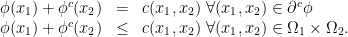
The demand that we should carry all of the mass in to reach all of is formulated by marginals. For simplicity we just write these constraints as

(with the understanding that the first equation really means that for all continuous function  it holds that
  ).
).
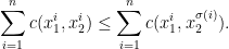
This leads us to the full transport problem

There is the following theorem which characterizes optimality of a plan and which is the topic of this post:
Theorem 1 (Fundamental theorem of optimal transport) Under some technicalities we can say that a plan which fulfills the marginal constraints is optimal if and only if one of the following equivalent conditions is satisfied:
- The support
 of is
of is  -cyclically monotone.
- There exists a -concave function
 such that its -superdifferential contains the support of , i.e.
  .
.
A few clarifications: The technicalities involve continuity, integrability, and boundedness conditions of and integrability conditions on the marginals. The full theorem can be found as Theorem 1.13 in A user’s guide to optimal transport by Ambrosio and Gigli. Also the notions -cyclically monotone, -concave and -superdifferential probably need explanation. We start with a simpler notion: -monotonicity:
Definition 2 A set  is -monotone, if for all
  it holds that

If you find it unclear what this has to do with monotonicity, look at this example:
Example 1 Let  and let
  be the usual scalar product. Then -monotonicity is the condition that for all
  it holds that

which may look more familiar. Indeed, when and are subset of the real line, the above conditions means that the set  somehow “moves up in ” if we “move right in ”. So -monotonicity for is something like “monotonically increasing”. Similarly, for
  , -monotonicity means “monotonically decreasing”.
You may say that both and are strange cost functions and I can’t argue with that. But here comes:  (
( being the euclidean norm) seems more natural, right? But if we have a transport plan for this for some marginals and we also have
i.e., the transport cost for differs from the one for only by a constant independent of , so may well use the latter.
The fundamental theorem of optimal transport uses the notion of -cyclical monotonicity which is stronger that just -monotonicity:
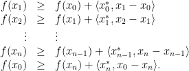
Definition 3 A set  is -cyclically monotone, if for all
  ,
,  and all permutations
  of
of  it holds that
For  we get back the notion of -monotonicity.
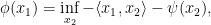
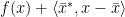
Definition 4 A function  is -concave if there exists some function
  such that
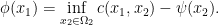
This definition of -concavity resembles the notion of convex conjugate:
Example 2 Again using we get that a function is -concave if
and, as an infimum over linear functions, is clearly concave in the usual way.
Definition 5 The -superdifferential of a -concave function is

where  is the -conjugate of defined by

Again one may look at and observe that the -superdifferential is the usual superdifferential related to the supergradient of concave functions (there is a Wikipedia page for subgradient only, but the concept is the same with reversed signs in some sense).
Now let us sketch the proof of the fundamental theorem of optimal transport: \medskip
Proof (of the fundamental theorem of optimal transport). Let be an optimal transport plan. We aim to show that is -cyclically monotone and assume the contrary. That is, we assume that there are points  and a permutation such that
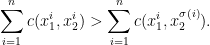
We aim to construct a  such that is still feasible but has a smaller transport cost. To do so, we note that continuity of implies that there are neighborhoods
  of
of  and
and  of
of  such that for all
  and
and  it holds that

We use this to construct a better plan  : Take the mass of in the sets
  and shift it around. The full construction is a little messy to write down: Define a probability measure
  on the product
 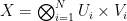 as the product of the measures
  . Now let
  and
and  be the projections of
  onto and , respectively, and set
where  denotes the pushforward of measures. Note that the new measure is signed and that
  fulfills
- is a non-negative measure
- is feasible, i.e. has the correct marginals
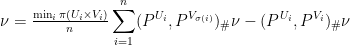
which, all together, gives a contradiction to optimality of . The implication of item 1 to item 2 of the theorem is not really related to optimal transport but a general fact about -concavity and -cyclical monotonicity (c.f.~this previous blog post of mine where I wrote a similar statement for convexity). So let us just prove the implication from item 2 to optimality of : Let fulfill item 2, i.e. is feasible and is contained in the -superdifferential of some -concave function . Moreover let be any feasible transport plan. We aim to show that 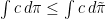 . By definition of the -superdifferential and the -conjugate we have
Since  by assumption, this gives
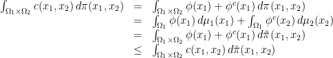
which shows the claim.

Corollary 6 If is a measure on which is supported on a -superdifferential of a -concave function, then is an optimal transport plan for its marginals with respect to the transport cost .


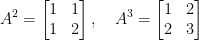
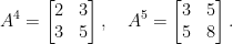


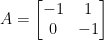
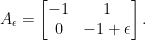


 . This matrix has
  as a double eigenvalue, but the corresponding eigenspace is one-dimensional and spanned by
  . To extend this vector to a basis we calculate a principle vector by solving

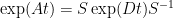
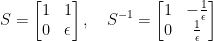
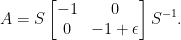
![{S = [v_{1}\, v_{2}]}](https://s0.wp.com/latex.php?latex=%7BS+%3D+%5Bv_%7B1%7D%5C%2C+v_%7B2%7D%5D%7D&bg=ffffff&fg=000000&s=0&c=20201002) we get the Jordan canonical form of
we get the Jordan canonical form of  as
as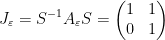

 is not the Jordan canonical form of
 does not seem to be invertible and indeed we get
 (which is my definition of diagonalizability). It does promise that
  and in fact
 and we denote it by
  ! (You probably have heard that before…) What does that mean numerically? Any matrix that you represent in floating point numbers is actually a representative of a whole bunch of matrices. Each entry is only known up to a certain precision. But this bunch of matrices does contain some matrix which is diagonalizable! This is exactly, what it means to be a dense set! So it is impossible to say if a matrix given in floating point numbers is actually diagonalizable or not. So, what matrix was diagonalized by MATLAB? Let us have closer look at the matrix
  :
: is indeed just the inverse of the machine precision, so this inverse is actually 100% accurate. Recombining gives
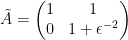


 .
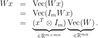
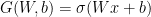
. where
where  is the weight matrix,
  is the bias,
  is the input, and
  ) and the function mapping
  which applies
  and
and  . So we need to take the derivative with respect to
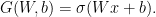
 is a concatenation of the map
 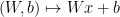 and
and  , the derivative of
  as linear maps in
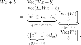
  . So let’s rewrite the thing:
![{W = [w_{1}\ \cdots\ w_{n}]}](https://s0.wp.com/latex.php?latex=%7BW+%3D+%5Bw_%7B1%7D%5C+%5Ccdots%5C+w_%7Bn%7D%5D%7D&bg=ffffff&fg=000000&s=0&c=20201002) and maps it by
and maps it by 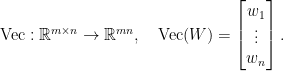
 and
and  is a matrix in

 ,
,  of compatible size we have that
 mapping
  can be rewritten as
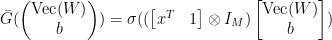
 . Since
  is just a concatenation of
  ) is calculated simply as
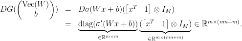
 (e.g. to produce a scalar loss that we can minimize), i.e. we consider the map
![\displaystyle \begin{array}{rcl} \nabla F( \begin{pmatrix} \mathrm{Vec}(W)\\b \end{pmatrix}) &=& D\bar G( \begin{pmatrix} \mathrm{Vec}(W)\\b \end{pmatrix})^{T} DL(G(Wx+b))^{T}\\ &=& ([x^{T}\ 1]\otimes I_{m})^{T}\mathrm{diag}(\sigma'(Wx+b))\nabla L(G(Wx+b))\\ &=& \underbrace{( \begin{bmatrix} x\\ 1 \end{bmatrix} \otimes I_{m})}_{\in{\mathbb R}^{(mn+m)\times m}}\underbrace{\mathrm{diag}(\sigma'(Wx+b))}_{\in{\mathbb R}^{m\times m}}\underbrace{\nabla L(G(Wx+b))}_{\in{\mathbb R}^{m}}. \end{array}](https://s0.wp.com/latex.php?latex=%5Cdisplaystyle++%5Cbegin%7Barray%7D%7Brcl%7D++%5Cnabla+F%28+%5Cbegin%7Bpmatrix%7D+%5Cmathrm%7BVec%7D%28W%29%5C%5Cb+%5Cend%7Bpmatrix%7D%29+%26%3D%26+D%5Cbar+G%28+%5Cbegin%7Bpmatrix%7D+%5Cmathrm%7BVec%7D%28W%29%5C%5Cb+%5Cend%7Bpmatrix%7D%29%5E%7BT%7D+DL%28G%28Wx%2Bb%29%29%5E%7BT%7D%5C%5C+%26%3D%26+%28%5Bx%5E%7BT%7D%5C+1%5D%5Cotimes+I_%7Bm%7D%29%5E%7BT%7D%5Cmathrm%7Bdiag%7D%28%5Csigma%27%28Wx%2Bb%29%29%5Cnabla+L%28G%28Wx%2Bb%29%29%5C%5C+%26%3D%26+%5Cunderbrace%7B%28+%5Cbegin%7Bbmatrix%7D+x%5C%5C+1+%5Cend%7Bbmatrix%7D+%5Cotimes+I_%7Bm%7D%29%7D_%7B%5Cin%7B%5Cmathbb+R%7D%5E%7B%28mn%2Bm%29%5Ctimes+m%7D%7D%5Cunderbrace%7B%5Cmathrm%7Bdiag%7D%28%5Csigma%27%28Wx%2Bb%29%29%7D_%7B%5Cin%7B%5Cmathbb+R%7D%5E%7Bm%5Ctimes+m%7D%7D%5Cunderbrace%7B%5Cnabla+L%28G%28Wx%2Bb%29%29%7D_%7B%5Cin%7B%5Cmathbb+R%7D%5E%7Bm%7D%7D.+%5Cend%7Barray%7D+&bg=ffffff&fg=000000&s=0&c=20201002)
 and hence, can be reshaped to a tupel
  matrix and an
  vector.
 and
and  , respectively, then
  represents the tensor product of the maps,
  . This relation to tensor products and tensors explains where the tensor in
  -Lipschitz +
  -strongly monotone, the iteration with stepsize
  converges linear with rate
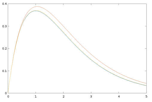
 there is a best
  and also a smallest contraction factor
  . Here are plots of these quantities:
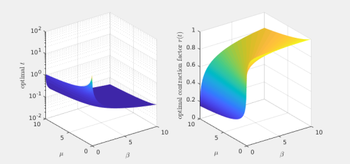

 from a Hilbert space into itself. Using the resolvent
  and the reflector
  , the Douglas-Rachford iteration is concisely written as
 is monotone if
  , we can introduce a stepsize for the Douglas-Rachford iteration
 and
and  -strongly monotone, than the Douglas-Rachford iterates converge strongly to a solution with a linear rate


 to get on optimal stepsize (in the sense that the guaranteed contraction factor is as small as possible). As Moursi and Vandenberghe explain in their Remark 5.4, this optimization involves finding the root of a polynomial of degree 5, so it is possible but cumbersome.
 in the case of single valued
  in the domain (which has to be an interval) and then set
 with
with  .
. is defined on a simply connected domain in
  we can recover
 from
from 
 is convex if for every
  such that for all
  one has the subgradient inequality
 as corresponding subgradient to
 is a (multivalued) monotone mapping. Recall that a multivalued map
  and
and  it holds that
 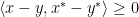 . It is not hard to see that not every monotone map is actually a subgradient of a convex function (not even, if we go to “maximally monotone maps”, a notion that we sweep under the rug in this post). A simple counterexample is a (singlevalued) linear monotone map represented by
 :
:

 -cyclical monotonicity. In these terms we can say that a subgradient of a convex function is cyclical monotone, which means that it is
  .
.  and set

 . As a supremum of affine functions
  since
since  everywhere). Finally, for
  we have
 and this shows that
 . Now consider a path
  with
with  . Then the term inside the supremum of~
 . By monotonicity of
  , we increase this sum, if we add another point
  (e.g.
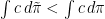
(e.g.  , and hence, the supremum does converge to the integral, i.e.~
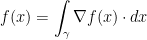
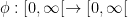 which satisfies
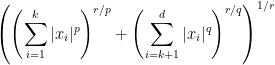
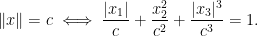
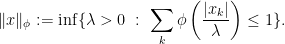
  and are increasing and convex (and thus, continuous). The definition of the Luxemburg norm in this case is
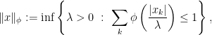
 if
if 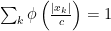 .
. are functions as
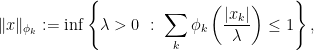
 if and only if
 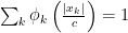 . The proof that this construction indeed gives a norm is the same as in the one in the previous post.
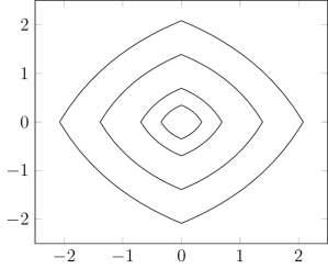
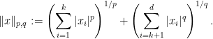
 -norms in different directions. Here is a simple example: In the case of
  we can split the variables into two groups, say the first
  variables. The first group shall be treated with a
  -norm. For the respective Luxemburg norm one has
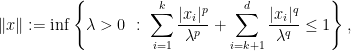
 functionals
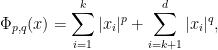
 .)
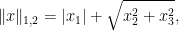
.) i.e., three-dimensional space, and picture the norm-balls (of level sets in the case the functionals
  and the first exponent to be
  and the second
  . The mixed norm is
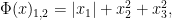

 :
:
 and the same exponents. This makes the mixed norm equal to the

 Again note how the Luxemburg ball keeps its shape while the level sets of the
  ,
,  and
and  . The mixed norm is again the
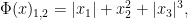
 . This implies that
  and thus, all
 .
.
 and
and 
 , then
  if and only if
  .
.  we have
  and for
  we have
  .
.  is a norm on
  we easily see that
  (since
  but since
  this can only hold if
  . For positive homogeneity observe
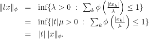
 (which implies that
  and
and  ). Then it follows
 as desired.
  lead to
  .
. .
.
 (which is not a norm):
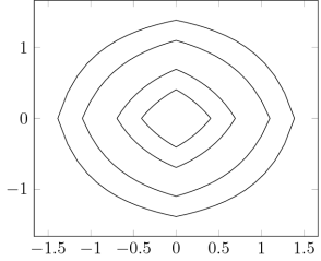
 ]
]