I blogged about the Douglas-Rachford method before and in this post I’d like to dig a bit into the history of the method.
As the name suggests, the method has its roots in a paper by Douglas and Rachford and the paper is
Douglas, Jim, Jr., and Henry H. Rachford Jr., “On the numerical solution of heat conduction problems in two and three space variables.” Transactions of the American mathematical Society 82.2 (1956): 421-439.
At first glance, the title does not suggest that the paper may be related to monotone inclusions and if you read the paper you’ll not find any monotone operator mentioned. So let’s start and look at Douglas and Rachford’s paper.
1. Solving the heat equation numerically
So let us see, what they were after and how this is related to what is known as Douglas-Rachford splitting method today.
Indeed, Douglas and Rachford wanted to solve the instationary heat equation

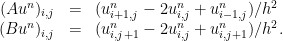
with Dirichlet boundary conditions (they also considered three dimensions, but let us skip that here). They considered a rectangular grid and a very simple finite difference approximation of the second derivatives, i.e.

(with modifications at the boundary to accomodate the boundary conditions). To ease notation, we abbreviate the difference quotients as operators (actually, also matrices) that act for a fixed time step
With this notation, our problem is to solve

in time.
Then they give the following iteration:


(plus boundary conditions which I’d like to swipe under the rug here). If we eliminate 

This is a kind of implicit Euler method with an additional small term 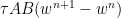


How do they prove convergence of the method? They don’t since they wanted to solve a parabolic PDE. They were after stability of the scheme, and this can be done by analyzing the eigenvalues of the iteration. Since the matrices
We reformulate the iteration (3) further to see how 


2. What about monotone inclusions?
What has the previous section to do with solving monotone inclusions? A monotone inclusion is

with a monotone operator, that is, a multivalued mapping 


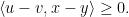
We are going to restrict ourselves to real Hilbert spaces here. Note that linear operators are monotone if they are positive semi-definite and further note that monotone linear operators need not to be symmetric. A general approach to the solution of monotone inclusions are so-called splitting methods. There one splits 

to obtain a numerical method. By the way, the resolvent of a monotone operator always exists and is single valued (to be honest, one needs a regularity assumption here, namely one need maximal monotone operators, but we will not deal with this issue here).
The two operators 


and write the iteration~(4) in terms of monotone operators as

i.e.

Using 

![\displaystyle \begin{array}{rcl} w^{n+1} & = &(I+\tau B)^{-1}[(I+\tau A)^{-1}(I-\tau B) + \tau B]w^{n}\\ & =& R_{\tau B}(R_{\tau A}(w^{n}-\tau Bw^{n}) + \tau Bw^{n}). \end{array}](https://s0.wp.com/latex.php?latex=%5Cdisplaystyle+%5Cbegin%7Barray%7D%7Brcl%7D+w%5E%7Bn%2B1%7D+%26+%3D+%26%28I%2B%5Ctau+B%29%5E%7B-1%7D%5B%28I%2B%5Ctau+A%29%5E%7B-1%7D%28I-%5Ctau+B%29+%2B+%5Ctau+B%5Dw%5E%7Bn%7D%5C%5C+%26+%3D%26+R_%7B%5Ctau+B%7D%28R_%7B%5Ctau+A%7D%28w%5E%7Bn%7D-%5Ctau+Bw%5E%7Bn%7D%29+%2B+%5Ctau+Bw%5E%7Bn%7D%29.+%5Cend%7Barray%7D+&bg=ffffff&fg=000000&s=0&c=20201002)
This is not really applicable to a general monotone inclusion since there 
But what to do, when both and 

We cancel the outer 


and here we go: This is exactly what is known as Douglas-Rachford method (see the last version of the iteration in my previous post). Note that it is not 


The observation, that these splitting method that Douglas and Rachford devised for linear problems has a kind of much wider applicability is due to Lions and Mercier and the paper is
Lions, Pierre-Louis, and Bertrand Mercier. “Splitting algorithms for the sum of two nonlinear operators.” SIAM Journal on Numerical Analysis 16.6 (1979): 964-979.
Other, much older, splitting methods for linear systems, such as the Jacobi method, the Gauss-Seidel method used different properties of the matrices such as the diagonal of the matrix or the upper and lower triangluar parts and as such, do not generalize easily to the case of operators on a Hilbert space.

June 6, 2018 at 9:28 am
[…] blogged about the Douglas-Rachford method before here and here. It’s a method to solve monotone inclusions in the […]