In my previous post I illustrated why it is not possible to compute the Jordan canonical form numerically (i.e. in floating point numbers). The simple reason: For every matrix 


with matrix 

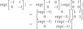
where the matrix exponential is
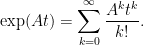
It is not always simple to work out the matrix exponential by hand. The straightforward way would be to calculate all the powers of 

Its first powers are
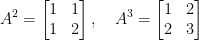
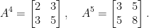
You may notice that the Fibonicci numbers appear (and this is pretty clear on a second thought). So, finding a explicit form for 

Another way is diagonalization: If 


you see that
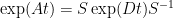
and the matrix exponential of a diagonal matrix is simply the exponential function applied to the diagonal entries.
But not all matrices are diagonalizable! The solution that is usually presented in the classroom is to use the Jordan canonical form instead and to compute the matrix exponential of Jordan blocks (using that you can split a Jordan block 


But in light of the fact that there are a diagonalizable matrices arbitrarily close to any matrix, on may ask: What about replacing a non-diagonalizable matrix
Let’s try this on a simple example:
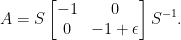
We consider
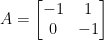
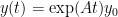
which is not diagonalizable. The linear initial value problem
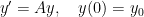
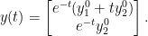
has the solution
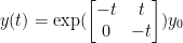
and the matrix exponential is
So we get the solution
Let us take a close-by matrix which is diagonalizable. For some small
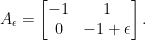
Since 
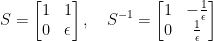
we get
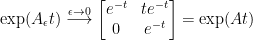
The matrix exponential of 

Hence, the solution of 

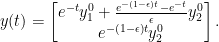
How is this related to the solution of 
Of course, the lower right entry of 


is nothing else that the (negative) difference quotient for the derivative of the function 

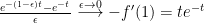
and we get
as expected.
It turns out that a fairly big 


to $\e

Leave a comment