The fundamental theorem of optimal transport

The problem of optimal transport of mass from one distribution to another can be stated in many forms. Here is the formulation going back to Kantorovich: We have two measurable sets ${\Omega_{1}}$ and ${\Omega_{2}}$ , coming with two measures ${\mu_{1}}$ and ${\mu_{2}}$ . We also have a function ${c:\Omega_{1}\times \Omega_{2}\rightarrow {\mathbb R}}$ which assigns a transport cost, i.e. ${c(x_{1},x_{2})}$ is the cost that it takes to carry one unit of mass from point ${x_{1}\in\Omega_{2}}$ to ${x_{2}\in\Omega_{2}}$ . What we want is a plan that says where the mass in ${\mu_{1}}$ should be placed in ${\Omega_{2}}$ (or vice versa). There are different ways to formulate this mathematically.

A simple way is to look for a map ${T:\Omega_{1}\rightarrow\Omega_{2}}$ which says that thet mass in ${x_{1}}$ should be moved to ${T(x_{1})}$ . While natural, there is a serious problem with this: What if not all mass at ${x_{1}}$ should go to the same point in ${\Omega_{2}}$ ? This happens in simple situations where all mass in ${\Omega_{1}}$ sits in just one point, but there are at least two different points in ${\Omega_{2}}$ where mass should end up. This is not going to work with a map ${T}$ as above. So, the map ${T}$ is not flexible enough to model all kinds of transport we may need.

What we want is a way to distribute mass from one point in ${\Omega_{1}}$ to the whole set ${\Omega_{2}}$ . This looks like we want maps ${\mathcal{T}}$ which map points in ${\Omega_{1}}$ to functions on ${\Omega_{2}}$ , i.e. something like ${\mathcal{T}:\Omega_{1}\rightarrow (\Omega_{2}\rightarrow{\mathbb R})}$ where ${(\Omega_{2}\rightarrow{\mathbb R})}$ stands for some set of functions on ${\Omega_{2}}$ . We can de-curry this function to some ${\tau:\Omega_{1}\times\Omega_{2}\rightarrow{\mathbb R}}$ by ${\tau(x_{1},x_{2}) = \mathcal{T}(x_{1})(x_{2})}$ . That’s good in principle, be we still run into problems when the target mass distribution ${\mu_{2}}$ is singular in the sense that ${\Omega_{2}}$ is a “continuous” set and there are single points in ${\Omega_{2}}$ that carry some mass according to ${\mu_{2}}$ . Since we are in the world of measure theory already, the way out suggests itself: Instead of a function ${\tau}$ on ${\Omega_{1}\times\Omega_{2}}$ we look for a measure ${\pi}$ on ${\Omega_{1}\times \Omega_{2}}$ as a transport plan.

The demand that we should carry all of the mass in ${\Omega_{1}}$ to reach all of ${\mu_{2}}$ is formulated by marginals. For simplicity we just write these constraints as

$\displaystyle \int_{\Omega_{2}}\pi\, d x_{2} = \mu_{1},\qquad \int_{\Omega_{1}}\pi\, d x_{1} = \mu_{2}$

(with the understanding that the first equation really means that for all continuous function ${f:\Omega_{1}\rightarrow {\mathbb R}}$ it holds that ${\int_{\Omega_{1}\times \Omega_{2}} f(x_{1})\,d\pi(x_{1},x_{2}) = \int_{\Omega_{1}}f(x_{1})\,d\mu_{1}(x_{1})}$ ).

This leads us to the full transport problem

$\displaystyle \min_{\pi}\int_{\Omega_{1}\times \Omega_{2}}c(x,y)\,d\pi(x_{1}x_{2})\quad \text{s.t.}\quad \int_{\Omega_{2}}\pi\, d x_{2} = \mu_{1},\quad \int_{\Omega_{1}}\pi\, d x_{1} = \mu_{2}.$

There is the following theorem which characterizes optimality of a plan and which is the topic of this post:

Theorem 1 (Fundamental theorem of optimal transport) Under some technicalities we can say that a plan ${\pi}$ which fulfills the marginal constraints is optimal if and only if one of the following equivalent conditions is satisfied:

The support ${\mathrm{supp}(\pi)}$ of ${\pi}$ is ${c}$ -cyclically monotone.

There exists a ${c}$ -concave function ${\phi}$ such that its ${c}$ -superdifferential contains the support of ${\pi}$ , i.e. ${\mathrm{supp}(\pi)\subset \partial^{c}\phi}$ .

A few clarifications: The technicalities involve continuity, integrability, and boundedness conditions of ${c}$ and integrability conditions on the marginals. The full theorem can be found as Theorem 1.13 in A user’s guide to optimal transport by Ambrosio and Gigli. Also the notions ${c}$ -cyclically monotone, ${c}$ -concave and ${c}$ -superdifferential probably need explanation. We start with a simpler notion: ${c}$ -monotonicity:

Definition 2 A set ${\Gamma\subset\Omega_{1}\times\Omega_{2}}$ is ${c}$ -monotone, if for all 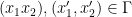${(x_{1}x_{2}),(x_{1}',x_{2}')\in\Gamma}$ it holds that

$\displaystyle c(x_{1},x_{2}) + c(x_{1}',x_{2}')\leq c(x_{1},x_{2}') + c(x_{1}',x_{2}).$

If you find it unclear what this has to do with monotonicity, look at this example:

Example 1 Let ${\Omega_{1/2}\in{\mathbb R}^{d}}$ and let ${c(x_{1},x_{2}) = \langle x_{1},x_{2}\rangle}$ be the usual scalar product. Then ${c}$ -monotonicity is the condition that for all ${(x_{1}x_{2}),(x_{1}',x_{2}')\in\Gamma\subset\Omega_{1}\times\Omega_{2}}$ it holds that

$\displaystyle 0\leq \langle x_{1}-x_{1}',x_{2}-x_{2}'\rangle$

which may look more familiar. Indeed, when ${\Omega_{1}}$ and ${\Omega_{2}}$ are subset of the real line, the above conditions means that the set ${\Gamma}$ somehow “moves up in ${\Omega_{2}}$ ” if we “move right in ${\Omega_{1}}$ ”. So ${c}$ -monotonicity for ${c(x_{1},x_{2}) = \langle x_{1},x_{2}\rangle}$ is something like “monotonically increasing”. Similarly, for ${c(x_{1},x_{2}) = -\langle x_{1},x_{2}\rangle}$ , ${c}$ -monotonicity means “monotonically decreasing”.

You may say that both ${c(x_{1},x_{2}) = \langle x_{1},x_{2}\rangle}$ and ${c(x_{1},x_{2}) = -\langle x_{1},x_{2}\rangle}$ are strange cost functions and I can’t argue with that. But here comes: 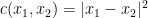${c(x_{1},x_{2}) = |x_{1}-x_{2}|^{2}}$ ( ${|\,\cdot\,|}$ being the euclidean norm) seems more natural, right? But if we have a transport plan ${\pi}$ for this ${c}$ for some marginals ${\mu_{1}}$ and ${\mu_{2}}$ we also have

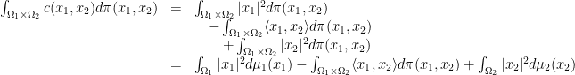
$\displaystyle \begin{array}{rcl} \int_{\Omega_{1}\times \Omega_{2}}c(x_{1},x_{2})d\pi(x_{1},x_{2}) & = & \int_{\Omega_{1}\times \Omega_{2}}|x_{1}|^{2} d\pi(x_{1},x_{2})\\ &&\quad- \int_{\Omega_{1}\times \Omega_{2}}\langle x_{1},x_{2}\rangle d\pi(x_{1},x_{2})\\ && \qquad+ \int_{\Omega_{1}\times \Omega_{2}} |x_{2}|^{2}d\pi(x_{1},x_{2})\\ & = &\int_{\Omega_{1}}|x_{1}|^{2}d\mu_{1}(x_{1}) - \int_{\Omega_{1}\times \Omega_{2}}\langle x_{1},x_{2}\rangle d\pi(x_{1},x_{2}) + \int_{\Omega_{2}}|x_{2}|^{2}d\mu_{2}(x_{2}) \end{array}$

i.e., the transport cost for ${c(x_{1},x_{2}) = |x_{1}-x_{2}|^{2}}$ differs from the one for ${c(x_{1},x_{2}) = -\langle x_{1},x_{2}\rangle}$ only by a constant independent of ${\pi}$ , so may well use the latter.

The fundamental theorem of optimal transport uses the notion of ${c}$ -cyclical monotonicity which is stronger that just ${c}$ -monotonicity:

Definition 3 A set ${\Gamma\subset \Omega_{1}\times \Omega_{2}}$ is ${c}$ -cyclically monotone, if for all ${(x_{1}^{i},x_{2}^{i})\in\Gamma}$ , ${i=1,\dots n}$ and all permutations ${\sigma}$ of ${\{1,\dots,n\}}$ it holds that

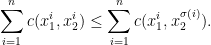
$\displaystyle \sum_{i=1}^{n}c(x_{1}^{i},x_{2}^{i}) \leq \sum_{i=1}^{n}c(x_{1}^{i},x_{2}^{\sigma(i)}).$

For ${n=2}$ we get back the notion of ${c}$ -monotonicity.

Definition 4 A function ${\phi:\Omega_{1}\rightarrow {\mathbb R}}$ is ${c}$ -concave if there exists some function ${\psi:\Omega_{2}\rightarrow{\mathbb R}}$ such that

$\displaystyle \phi(x_{1}) = \inf_{x_{2}\in\Omega_{2}}c(x_{1},x_{2}) - \psi(x_{2}).$

This definition of ${c}$ -concavity resembles the notion of convex conjugate:

Example 2 Again using ${c(x_{1},x_{2}) = -\langle x_{1},x_{2}\rangle}$ we get that a function ${\phi}$ is ${c}$ -concave if

$\displaystyle \phi(x_{1}) = \inf_{x_{2}}-\langle x_{1},x_{2}\rangle - \psi(x_{2}),$

and, as an infimum over linear functions, ${\phi}$ is clearly concave in the usual way.

Definition 5 The ${c}$ -superdifferential of a ${c}$ -concave function is

$\displaystyle \partial^{c}\phi = \{(x_{1},x_{2})\mid \phi(x_{1}) + \phi^{c}(x_{2}) = c(x,y)\},$

where ${\phi^{c}}$ is the ${c}$ -conjugate of ${\phi}$ defined by

$\displaystyle \phi^{c}(x_{2}) = \inf_{x_{1}\in\Omega_{1}}c(x_{1},x_{2}) -\phi(x_{1}).$

Again one may look at ${c(x_{1},x_{2}) = -\langle x_{1},x_{2}\rangle}$ and observe that the ${c}$ -superdifferential is the usual superdifferential related to the supergradient of concave functions (there is a Wikipedia page for subgradient only, but the concept is the same with reversed signs in some sense).

Now let us sketch the proof of the fundamental theorem of optimal transport: \medskip

Proof (of the fundamental theorem of optimal transport). Let ${\pi}$ be an optimal transport plan. We aim to show that ${\mathrm{supp}(\pi)}$ is ${c}$ -cyclically monotone and assume the contrary. That is, we assume that there are points ${(x_{1}^{i},x_{2}^{i})\in\mathrm{supp}(\pi)}$ and a permutation ${\sigma}$ such that

$\displaystyle \sum_{i=1}^{n}c(x_{1}^{i},x_{2}^{i}) > \sum_{i=1}^{n}c(x_{1}^{i},x_{2}^{\sigma(i)}).$

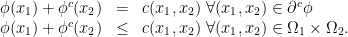
We aim to construct a ${\tilde\pi}$ such that ${\tilde\pi}$ is still feasible but has a smaller transport cost. To do so, we note that continuity of ${c}$ implies that there are neighborhoods ${U_{i}}$ of ${x_{1}^{i}}$ and ${V_{i}}$ of ${x_{2}^{i}}$ such that for all ${u_{i}\in U_{1}}$ and ${v_{i}\in V_{i}}$ it holds that

$\displaystyle \sum_{i=1}^{n}c(u_{i},v_{\sigma(i)}) - c(u_{i},v_{i})<0.$

We use this to construct a better plan ${\tilde \pi}$ : Take the mass of ${\pi}$ in the sets ${U_{i}\times V_{i}}$ and shift it around. The full construction is a little messy to write down: Define a probability measure ${\nu}$ on the product ${X = \bigotimes_{i=1}^{N}U_{i}\times V_{i}}$ as the product of the measures ${\tfrac{1}{\pi(U_{i}\times V_{i})}\pi|_{U_{i}\times V_{i}}}$ . Now let ${P^{U_{1}}}$ and ${P^{V_{i}}}$ be the projections of ${X}$ onto ${U_{i}}$ and ${V_{i}}$ , respectively, and set

$\displaystyle \nu = \tfrac{\min_{i}\pi(U_{i}\times V_{i})}{n}\sum_{i=1}^{n}(P^{U_{i}},P^{V_{\sigma(i)}})_{\#}\nu - (P^{U_{i}},P^{V_{i}})_{\#}\nu$

where ${_{\#}}$ denotes the pushforward of measures. Note that the new measure ${\nu}$ is signed and that ${\tilde\pi = \pi + \nu}$ fulfills

${\tilde\pi}$ is a non-negative measure
${\tilde\pi}$ is feasible, i.e. has the correct marginals
${\int c\,d\tilde \pi<\int c\,d\pi}$

which, all together, gives a contradiction to optimality of ${\pi}$ . The implication of item 1 to item 2 of the theorem is not really related to optimal transport but a general fact about ${c}$ -concavity and ${c}$ -cyclical monotonicity (c.f.~this previous blog post of mine where I wrote a similar statement for convexity). So let us just prove the implication from item 2 to optimality of ${\pi}$ : Let ${\pi}$ fulfill item 2, i.e. ${\pi}$ is feasible and ${\mathrm{supp}(\pi)}$ is contained in the ${c}$ -superdifferential of some ${c}$ -concave function ${\phi}$ . Moreover let ${\tilde\pi}$ be any feasible transport plan. We aim to show that ${\int c\,d\pi\leq \int c\,d\tilde\pi}$ . By definition of the ${c}$ -superdifferential and the ${c}$ -conjugate we have

$\displaystyle \begin{array}{rcl} \phi(x_{1}) + \phi^{c}(x_{2}) &=& c(x_{1},x_{2})\ \forall (x_{1},x_{2})\in\partial^{c}\phi\\ \phi(x_{1}) + \phi^{c}(x_{2}) & \leq& c(x_{1},x_{2})\ \forall (x_{1},x_{2})\in\Omega_{1}\times \Omega_{2}. \end{array}$

Since ${\mathrm{supp}(\pi)\subset\partial^{c}\phi}$ by assumption, this gives

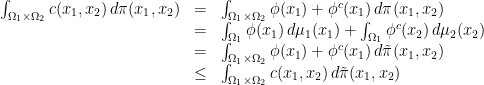
$\displaystyle \begin{array}{rcl} \int_{\Omega_{1}\times \Omega_{2}}c(x_{1},x_{2})\,d\pi(x_{1},x_{2}) & =& \int_{\Omega_{1}\times \Omega_{2}}\phi(x_{1}) + \phi^{c}(x_{1})\,d\pi(x_{1},x_{2})\\ &=& \int_{\Omega_{1}}\phi(x_{1})\,d\mu_{1}(x_{1}) + \int_{\Omega_{1}}\phi^{c}(x_{2})\,d\mu_{2}(x_{2})\\ &=& \int_{\Omega_{1}\times \Omega_{2}}\phi(x_{1}) + \phi^{c}(x_{1})\,d\tilde\pi(x_{1},x_{2})\\ &\leq& \int_{\Omega_{1}\times \Omega_{2}}c(x_{1},x_{2})\,d\tilde\pi(x_{1},x_{2}) \end{array}$

which shows the claim.

${\Box}$

Corollary 6 If ${\pi}$ is a measure on ${\Omega_{1}\times \Omega_{2}}$ which is supported on a ${c}$ -superdifferential of a ${c}$ -concave function, then ${\pi}$ is an optimal transport plan for its marginals with respect to the transport cost ${c}$ .

regularize