How many samples are needed to reconstruct a sparse signal?
Well, there are many, many results around some of which you probably know (at least if you are following this blog or this one). Today I write about a neat result which I found quite some time ago on reconstruction of nonnegative sparse signals from a semi-continuous perspective.
1. From discrete sparse reconstruction/compressed sensing to semi-continuous
The basic sparse reconstruction problem asks the following: Say we have a vector  which only has
  non-zero entries and a fat matrix
  (i.e.
(i.e.  ) and consider that we are given measurements
  . Of course, the system
  is underdetermined. However, we may add a little more prior knowledge on the solution and ask: Is is possible to reconstruct
  from
from  if we know that the vector is sparse? If yes: How? Under what conditions on
  ,
,  ,
,  and
and  ? This question created the expanding universe of compressed sensing recently (and this universe is expanding so fast that for sure there has to be some dark energy in it). As a matter of fact, a powerful method to obtain sparse solutions to underdetermined systems is
  -minimization a.k.a. Basis Pursuit on which I blogged recently: Solve

and the important ingredient here is the -norm of the vector in the objective function.
In this post I’ll formulate semi-continuous sparse reconstruction. We move from an -vector to a finite signed measure  on a closed interval (which we assume to be
 ![{I=[-1,1]}](https://s0.wp.com/latex.php?latex=%7BI%3D%5B-1%2C1%5D%7D&bg=ffffff&fg=000000&s=0&c=20201002) for simplicty). We may embed the -vectors into the space of finite signed measures by choosing points
for simplicty). We may embed the -vectors into the space of finite signed measures by choosing points  ,
,  from the interval
  and build
 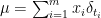 with the point-masses (or Dirac measures)
  . To a be a bit more precise, we speak about the space
  of Radon measures on , which are defined on the Borel
  -algebra of and are finite. Radon measures are not very scary objects and an intuitive way to think of them is to use Riesz representation: Every Radon measure arises as a continuous linear functional on a space of continuous functions, namely the space
  which is the closure of the continuous functions with compact support in
 ![{{]{-1,1}[}}](https://s0.wp.com/latex.php?latex=%7B%7B%5D%7B-1%2C1%7D%5B%7D%7D&bg=ffffff&fg=000000&s=0&c=20201002) with respect to the supremum norm. Hence, Radon measures work on these functions as
with respect to the supremum norm. Hence, Radon measures work on these functions as  . It is also natural to speak of the support
  of a Radon measure and it holds for any continuous function
  that
that

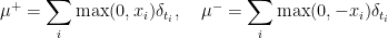
An important tool for Radon measures is the Hahn-Jordan decomposition which decomposes into a positive part  and a negative part
  , i.e. and are non-negative and
  . Finally the variation of a measure, which is

provides a norm on the space of Radon measures.
Example 1 For the measure one readily calculates that
and hence
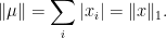
In this sense, the space of Radon measures provides a generalization of .
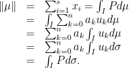
We may sample a Radon measure with  linear functionals and these can be encoded by continuous functions
  as
as

This sampling gives a bounded linear operator  . The generalization of Basis Pursuit is then given by
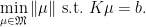
This was introduced and called “Support Pursuit” in the preprint Exact Reconstruction using Support Pursuit by Yohann de Castro and Frabrice Gamboa.
More on the motivation and the use of Radon measures for sparsity can be found in Inverse problems in spaces of measures by Kristian Bredies and Hanna Pikkarainen.
2. Exact reconstruction of sparse nonnegative Radon measures
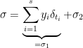
Before I talk about the results we may count the degrees of freedom a sparse Radon measure has: If  with some than is defined by the weights
  and the positions . Hence, we expect that at least
  linear measurements should be necessary to reconstruct . Surprisingly, this is almost enough if we know that the measure is nonnegative! We only need one more measurement, that is
  and moreover, we can take fairly simple measurements, namely the monomials:
 (with the convention that
  ). This is shown in the following theorem by de Castro and Gamboa.
Theorem 1 Let  with
with  ,
,  and let
  ,
,  be the monomials as above. Define
  . Then is the unique solution of the support pursuit problem, that is of

Proof: The following polynomial will be of importance: For a constant  define
The following properties of  will be used:
-
 for
for 
- has degree and hence, is a linear combination of the ,
 , i.e.
 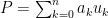 .
.
- For
 small enough it holds for
  that
that  .
.
Now let be a solution of (SP). We have to show that  . Due to property 2 we know that

Due to property 1 and non-negativity of we conclude that
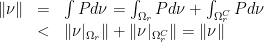
Moreover, by Lebesgue’s decomposition we can decompose with respect to such that
and  is singular with respect to . We get

and we conclude that  and especially
 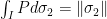 . This shows that is a solution to
  . It remains to show uniqueness. We show the following: If there is a
  with support in
  such that
  , then
  . To see this, we build, for any
  , the sets
![\displaystyle \Omega_r = [-1,1]\setminus \bigcup_{i=1}^s ]x_i-r,x_i+r[.](https://s0.wp.com/latex.php?latex=%5Cdisplaystyle++%5COmega_r+%3D+%5B-1%2C1%5D%5Csetminus+%5Cbigcup_%7Bi%3D1%7D%5Es+%5Dx_i-r%2Cx_i%2Br%5B.+&bg=ffffff&fg=000000&s=0&c=20201002)
and assume that there exists such that  (
( denoting the restriction of
  to
to  ). However, it holds by property 3 of that

and consequently
which is a contradiction. Hence,  for all
  and this implies . Since has its support in we conclude that
  . Hence the support of is exactly
  . and since
  and hence
  . This can be written as a Vandermonde system

which only has the zero solution, giving  .
. 
3. Generalization to other measurements
The measurement by monomials may sound a bit unusual. However, de Castro and Gamboa show more. What really matters here is that the monomials for a so-called Chebyshev-System (or Tchebyscheff-system or T-system – by the way, have you ever tried to google for a T-system?). This is explained, for example in the book “Tchebycheff Systems: With Applications in Analysis and Statistics” by Karlin and Studden. A T-system on is simply a set of functions  such that any linear combination of these functions has at most zeros. These systems are called after Tchebyscheff since they obey many of the helpful properties of the Tchebyscheff-polynomials.
What is helpful in our context is the following theorem of Krein:
Theorem 2 (Krein) If  is a T-system for ,
  and
and  are in the interior of , then there exists a linear combination
  which is non-negative and vanishes exactly the the point .
Now consider that we replace the monomials in Theorem~1 by a T-system. You recognize that Krein’s Theorem allows to construct a “generalized polynomial” which fulfills the same requirements than the polynomial is the proof of Theorem~1 as soon as the constant function 1 lies in the span of the T-system and indeed the result of Theorem~1 is also valid in that case.
4. Exact reconstruction of -sparse nonnegative vectors from measurements
From the above one can deduce a reconstruction result for -sparse vectors and I quote Theorem 2.4 from Exact Reconstruction using Support Pursuit:
Theorem 3 Let , , be integers such that  and let
  be a complete T-system on (that is,
  is a T-system on for all
  ). Then it holds: For any distinct reals
  and defined as

Basis Pursuit recovers all nonnegative -sparse vectors .
5. Concluding remarks
Note that Theorem~3 gives a deterministic construction of a measurement matrix.
Also note, that nonnegativity is crucial in what we did here. This allowed (in the monomial case) to work with squares and obtain the polynomial in the proof of Theorem~1 (which is also called “dual certificate” in this context). This raises the question how this method can be adapted to all sparse signals. One needs (in the monomial case) a polynomial which is bounded by 1 but matches the signs of the measure on its support. While this can be done (I think) for polynomials it seems difficult to obtain a generalization of Krein’s Theorem to this case…


with
induces a probability measure via
-measures: For every
there is the


is the set of convex combinations of the measures
(

,
and suppose that the subset
of

such that

we have


 system of equations. He formulated this as a feasibility-problem (well,
  the number of non-zero entries of
  . Then the problem of finding an
 -norm” is definitely not convex. One of the simplest algorithms for the convex feasibility problem is to alternatingly project onto both sets. This algorithm dates back to von Neumann and has been analyzed in great detail. To make this method work for non-convex sets one only needs to know how to project onto both sets. For the case of the equality constraint
  consists of just keeping the
  and
and  of which you observe only the superposition of
  you observe

 and
and 
 such that the residual (could also say “noise”)
  is also sparse. This differs from the common Basis Pursuit Denoising (BPDN) by the structure function for the residual (which is the squared
  -norm). This is due to the fact that in BPDN one usually assumes Gaussian noise which naturally lead to the squared
  is known.
 -norm (which is “non-smooth”) in contrast to the smooth
  , respectively. Assuming a kind of non-smoothness of
  . However, if the sparsity
  , which is a sharp lower bound on
  , and use non-asymptotic methods to bound the relative error of
  . These results also extend naturally to the problem of using linear measurements to estimate the rank of a positive semi-definite matrix, or the sparsity of a non-negative matrix. Finally, we show that if no structural assumption (such as non-negativity) is made on the signal
  cannot generally be estimated when
  . Similarly, measuring with Gaussian random vector you can obtain an estimate of
  .
. with Lipschitz-differentiable
  to second order Newton-type methods. The abstract reads
 is a convex but not necessarily differentiable function whose proximal mapping can be evaluated efficiently. We derive a generalization of Newton-type methods to handle such convex but nonsmooth objective functions. Many problems of relevance in high-dimensional statistics, machine learning, and signal processing can be formulated in composite form. We prove such methods are globally convergent to a minimizer and achieve quadratic rates of convergence in the vicinity of a unique minimizer. We also demonstrate the performance of such methods using problems of relevance in machine learning and high-dimensional statistics.