Some years ago I became fascinated by uncertainty principles. I got to know them via signal processing and not via physics, although, from a mathematical point of view they are the same.
I recently supervised a Master’s thesis on this topic and the results clarified a few things for me which I used to find obscure and I’d like to illustrate this here on my blog. However, it takes some space to introduce notation and to explain what it’s all about and hence, I decided to write a short series of posts, I try to explain, what new insights I got from the thesis. Here comes the first post:
1. The Fourier transform and the windowed Fourier transform
Let’s start with an important tool from signal processing you all know: The Fourier transform. For 

(I was tempted to say “whenever the integral is defined”. However, the details here are a little bit more involved, but I will not go into detail here; 


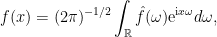
i.e. the (complex) number 


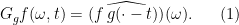
One drawback of the Fourier transform, when used to analyze signals, is its “global” nature in that the value 


is called windowed Fourier transform, short-time Fourier transform or (in the case of 
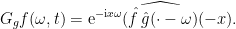
Of course we can write the windowed Fourier transform in term of the usual Fourier transform as
In other words: The localization in time is precisely determined by the “locality” of 


For the localization in frequency one obtains (by Plancherel’s formula and integral substitution) that
In other words: The localization in frequency is precisely determined by the “locality” of 
Hence, it seems clear that a function
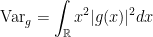
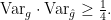
then there is the fundamental lower bound on the product of the variance of a function and the variance of its Fourier transform, know under the name “Heisenberg uncertainty principle” (or, as I learned from Wikipedia, “Gabor limit”): For 
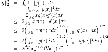
Proof: A simple (not totally rigorous) proof goes like this: We use partial integration, the Cauchy-Schwarz inequality and the Plancherel formula:

Moreover, the inequality is sharp for the functions 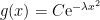

While this presentation was geared towards usability, there is a quite different approach to uncertainty principles related to integral transforms which uses the underlying group structure.
2. The group behind the windowed Fourier transform
The windowed Fourier transform (1) can also be seen as taking inner products of 
Definition 1 The Weyl-Heisenberg group
is the set
endowed with the operation

The Weyl-Heisenberg group admits a representation of the space of unitary operators on 


It indeed the operators 

Moreover, the mapping 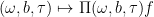
In this light, the windowed Fourier transform can be written as

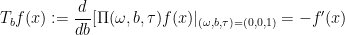
Now there is a motivation for the uncertainty principle as follows: Associated to the Weyl-Heisenberg group there is the Weyl-Heisenberg algebra, a basis of which is given by the so called infinitesimal generators. These are, roughly speaking, the derivatives of the representation with respect to the group parameters, evaluated at the identity. In the Weyl-Heisenberg case:

and
and
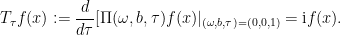
(In the last case, my notation was not too good: Note that 

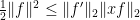
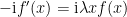
All these operators are skew adjoint on

are self adjoint.
For any two (possibly unbounded) operators on a Hilbert space there is a kind of abstract uncertainty principle (apparently sometimes known as Robertson’s uncertainty principle. It uses the commutator ![{[A,B] = AB-BA}](https://s0.wp.com/latex.php?latex=%7B%5BA%2CB%5D+%3D+AB-BA%7D&bg=ffffff&fg=000000&s=0&c=20201002)
Theorem 2 For any two self adjoint operators
and
on a Hilbert space it holds that for any
and any real numbers
and
it holds that
![\displaystyle \tfrac12|\langle [A,B] f,f\rangle|\leq \|(A-\mu_1 I)f\|\,\|(B-\mu_2)f\|.](https://s0.wp.com/latex.php?latex=%5Cdisplaystyle++%5Ctfrac12%7C%5Clangle+%5BA%2CB%5D+f%2Cf%5Crangle%7C%5Cleq+%5C%7C%28A-%5Cmu_1+I%29f%5C%7C%5C%2C%5C%7C%28B-%5Cmu_2%29f%5C%7C.+&bg=ffffff&fg=000000&s=0&c=20201002)
Proof: The proof simply consists of noting that
![\displaystyle \begin{array}{rcl} |\langle [A,B] f,f\rangle| &=& |\langle B f,Af\rangle -\langle Af,BS f\rangle|\\ & =& |\langle (B-\mu_2 I) f,(A-\mu_1 I)f\rangle -\langle (A-\mu_1 I)f,(B-\mu_2 I)S f\rangle|\\ & =& |2\text{Im} \langle (B-\mu_2 I) f,(A-\mu_1 I)f\rangle|\\ & \leq &2|\langle (B-\mu_2 I) f,(A-\mu_1 I)f\rangle|. \end{array}](https://s0.wp.com/latex.php?latex=%5Cdisplaystyle++%5Cbegin%7Barray%7D%7Brcl%7D++%7C%5Clangle+%5BA%2CB%5D+f%2Cf%5Crangle%7C+%26%3D%26+%7C%5Clangle+B+f%2CAf%5Crangle+-%5Clangle+Af%2CBS+f%5Crangle%7C%5C%5C+%26+%3D%26+%7C%5Clangle+%28B-%5Cmu_2+I%29+f%2C%28A-%5Cmu_1+I%29f%5Crangle+-%5Clangle+%28A-%5Cmu_1+I%29f%2C%28B-%5Cmu_2+I%29S+f%5Crangle%7C%5C%5C+%26+%3D%26+%7C2%5Ctext%7BIm%7D+%5Clangle+%28B-%5Cmu_2+I%29+f%2C%28A-%5Cmu_1+I%29f%5Crangle%7C%5C%5C+%26+%5Cleq+%262%7C%5Clangle+%28B-%5Cmu_2+I%29+f%2C%28A-%5Cmu_1+I%29f%5Crangle%7C.+%5Cend%7Barray%7D+&bg=ffffff&fg=000000&s=0&c=20201002)
Now use Cauchy-Schwarz to obtain the result.
Looking closer at the inequalities in the proof, one infers in which cases Robertson’s uncertainty principle is sharp: Precisely if there is a real 

Now the three self-adjoint operators 


![\displaystyle [\mathrm{i} T_b,\mathrm{i} T_\omega] f = \mathrm{i} f.](https://s0.wp.com/latex.php?latex=%5Cdisplaystyle++%5B%5Cmathrm%7Bi%7D+T_b%2C%5Cmathrm%7Bi%7D+T_%5Comega%5D+f+%3D+%5Cmathrm%7Bi%7D+f.+&bg=ffffff&fg=000000&s=0&c=20201002)
Hence, using 


which is exactly the Heisenberg uncertainty principle.
Moreover, by (2), equality happens if
the solution of which are exactly the functions 
Since the Heisenberg uncertainty principle is such an impressing thing with a broad range of implications (a colleague said that its interpretation, consequences and motivation somehow form a kind of “holy grail” in some communities), one may try to find other cool uncertainty principles be generalizing the approach of the previous sections to other transformations.
In the next post I am going to write about other group related integral transforms and its “uncertainty principles”.

September 18, 2011 at 6:00 pm
This is interesting. Looking forward to the next installment.
September 20, 2011 at 3:19 am
[…] while Azimuth studied Fool’s Gold. Flavors and Seasons shared a reflection on discussions and Regularize started a series on the uncertainty principle for the windowed Fourier transform. On top of that, […]
September 20, 2011 at 9:57 am
[…] my previous post on the uncertainty principle for the windowed Fourier transform, we now come to another integral […]
September 26, 2011 at 8:51 am
[…] last post on uncertainty principles will be probably the hardest one for me. As said in my first post, I supervised a Master’s thesis and posed the very vague question “Why are the […]
June 5, 2022 at 9:27 am
[…] consideration about uncertainty principle associated to group-related integral transforms (see my two blog posts). Interestingly, the Heisenberg uncertainty principle derived from the short time […]