The Kurdyka-Łojasiewicz inequality and gradient descent methods

The mother example of optimization is to solve problems

$\displaystyle \min_{x\in C} f(x)$

for functions ${f:{\mathbb R}^n\rightarrow{\mathbb R}}$ and sets ${C\in{\mathbb R}^n}$ . One further classifies problems according to additional properties of ${f}$ and ${C}$ : If ${C={\mathbb R}^n}$ one speaks of unconstrained optimization, if ${f}$ is smooth one speaks of smooth optimization, if ${f}$ and ${C}$ are convex one speaks of convex optimization and so on.

1. Classification, goals and accuracy

Usually, optimization problems do not have a closed form solution. Consequently, optimization is not primarily concerned with calculating solutions to optimization problems, but with algorithms to solve them. However, having a convergent or terminating algorithm is not fully satisfactory without knowing an upper bound on the runtime. There are several concepts one can work with in this respect and one is the iteration complexity. Here, one gives an upper bound on the number of iterations (which are only allowed to use certain operations such as evaluations of the function ${f}$ , its gradient ${\nabla f}$ , its Hessian, solving linear systems of dimension ${n}$ , projecting onto ${C}$ , calculating halfspaces which contain ${C}$ , or others) to reach a certain accuracy. But also for the notion of accuracy there are several definitions:

For general problems one can of course desire to be within a certain distance to the optimal point ${x^*}$ , i.e. ${\|x-x^*\|\leq \epsilon}$ for the solution ${x^*}$ and a given point ${x}$ .
One could also demand that one wants to be at a point which has a function value close to the optimal one ${f^*}$ , i.e, ${f(x) - f^*\leq \epsilon}$ . Note that for this and for the first point one could also desire relative accuracy.
For convex and unconstrained problems, one knowns that the inclusion ${0\in\partial f(x^*)}$ (with the subgradient ${\partial f(x)}$ ) characterizes the minimizers and hence, accuracy can be defined by desiring that ${\min\{\|\xi\|\ :\ \xi\in\partial f(x)\}\leq \epsilon}$ .

It turns out that the first two definitions of accuracy are much to hard to obtain for general problems and even for smooth and unconstrained problems. The main issue is that for general functions one can not decide if a local minimizer is also a solution (i.e. a global minimizer) by only considering local quantities. Hence, one resorts to different notions of accuracy, e.g.

For a smooth, unconstrained problems aim at stationary points, i.e. find ${x}$ such that ${\|\nabla f(x)\|\leq \epsilon}$ .
For smoothly constrained smooth problems aim at “approximately KKT-points” i.e. a point that satisfies the Karush-Kuhn-Tucker conditions approximately.

(There are adaptions to the nonsmooth case that are in the same spirit.) Hence, it would be more honest not write ${\min_x f(x)}$ in these cases since this is often not really the problem one is interested in. However, people write “solve ${\min_x f(x)}$ ” all the time even if they only want to find “approximately stationary points”.

2. The gradient method for smooth, unconstrainted optimization

Consider a smooth function ${f:{\mathbb R}^n\rightarrow {\mathbb R}}$ (we’ll say more precisely how smooth in a minute). We make no assumption on convexity and hence, we are only interested in finding stationary points. From calculus in several dimensions it is known that ${-\nabla f(x)}$ is a direction of descent from the point ${x}$ , i.e. there is a value ${h>0}$ such that 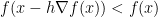${f(x - h\nabla f(x))< f(x)}$ . Hence, it seems like moving into the direction of the negative gradient is a good idea. We arrive at what is known as gradient method:

$\displaystyle x_{k+1} = x_k - h_k \nabla f(x_k).$

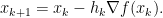
Now let’s be more specific about the smoothness of ${f}$ . Of course we need that ${f}$ is differentiable and we also want the gradient to be continuous (to make the evaluation of ${\nabla f}$ stable). It turns out that some more smoothness makes the gradient method more efficient, namely we require that the gradient of ${f}$ is Lipschitz continuous with a known Lipschitz constant ${L}$ . The Lipschitz constant can be used to produce efficient stepsizes ${h_k}$ , namely, for ${h_k = 1/L}$ one has the estimate

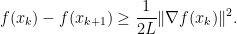
$\displaystyle f(x_k) - f(x_{k+1})\geq \frac{1}{2L}\|\nabla f(x_k)\|^2.$

This inequality is really great because one can use telescoping to arrive at

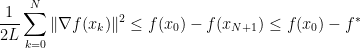
$\displaystyle \frac{1}{2L}\sum_{k=0}^N \|\nabla f(x_k)\|^2 \leq f(x_0) - f(x_{N+1}) \leq f(x_0) - f^*$

with the optimal value ${f}$ (note that we do not need to know ${f^*}$ for the following). We immediately arrive at

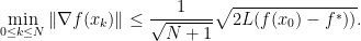
$\displaystyle \min_{0\leq k\leq N} \|\nabla f(x_k)\| \leq \frac{1}{\sqrt{N+1}}\sqrt{2L(f(x_0)-f^*))}.$

That’s already a result on the iteration complexity! Among the first ${N}$ iterates there is one which has a gradient norm of order ${N^{-1/2}}$ .

However, from here on it’s getting complicated: We can not say anything about the function values ${f(x_k)}$ and about convergence of the iterates ${x_k}$ . And even for convex functions ${f}$ (which allow for more estimates from above and below) one needs some more effort to prove convergence of the functional values to the global minimal one.

But how about convergence of the iterates for the gradient method if convexity is not given? It turns out that this is a hard problem. As illustration, consider the continuous case, i.e. a trajectory of the dynamical system

$\displaystyle \dot x = -\nabla f(x)$

(which is a continuous limit of the gradient method as the stepsize goes to zero). A physical intuition about this dynamical system in ${{\mathbb R}^2}$ is as follows: The function ${f}$ describes a landscape and ${x}$ are the coordinates of an object. Now, if the landscape is slippery the object slides down the landscape and if we omit friction and inertia, the object will always slide in the direction of the negative gradient. Consider now a favorable situation: ${f}$ is smooth, bounded from below and the level sets ${\{f\leq t\}}$ are compact. What can one say about the trajectories of the ${\dot x = -\nabla f(x)}$ ? Well, it seems clear that one will arrive at a local minimum after some time. But with a little imagination one can see that the trajectory of ${x}$ does not even has to be of finite length! To see this consider a landscape ${f}$ that is a kind of bowl-shaped valley with a path which goes down the hillside in a spiral way such that it winds around the minimum infinitely often. This situation seems somewhat pathological and one usually does not expect situation like this in practice. If you tried to prove convergence of the iterates of gradient or subgradient descent you may have noticed that one sometimes wonders why the proof turns out to be so complicated. The reason lies in the fact that such pathological functions are not excluded. But what functions should be excluded in order to avoid this pathological behavior without restricting to too simple functions?

3. The Kurdyka-Łojasiewicz inequality

Here comes the so-called Kurdyka-Łojasiewicz inequality into play. I do not know its history well, but if you want a pointer, you could start with the paper “On gradients of functions definable in o-minimal structures” by Kurdyka.

The inequality shall be a way to turn a complexity estimate for the gradient of a function into a complexity estimate for the function values. Hence, one would like to control the difference in functional value by the gradient. One way to do so is the following:

Definition 1 Let ${f}$ be a real valued function and assume (without loss of generality) that ${f}$ has a unique minimum at ${0}$ and that ${f(0)=0}$ . Then ${f}$ satisfies a Kurdyka-Łojasiewicz inequality if there exists a differentiable function ${\kappa:[0,r]\rightarrow {\mathbb R}}$ on some interval ${[0,r]}$ with ${\kappa'>0}$ and ${\kappa(0)=0}$ such that

$\displaystyle \|\nabla(\kappa\circ f)(x)\|\geq 1$

for all ${x}$ such that ${f(x)<r}$ .

Informally, this definition ensures that one can “reparameterize the range of the function such that the resulting function has a kink in the minimum and is steep around that minimum”. This definition is due to the above paper by Kurdyka from 1998. In fact it is a slight generalization of the Łowasiewicz inequality (which dates back to a note of Łojasiewicz from 1963) which states that there is some ${C>0}$ and some exponent ${\theta}$ such that in the above situation it holds that

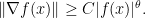
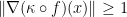
$\displaystyle \|\nabla f(x)\|\geq C|f(x)|^\theta.$

To see that, take ${\kappa(s) = s^{1-\theta}}$ and evaluate the gradient to ${\nabla(\kappa\circ f)(x) = (1-\theta)f(x)^{-\theta}\nabla f(x)}$ to obtain ${1\leq (1-\theta)|f(x)|^{-\theta}\|\nabla f(x)\|}$ . This also makes clear that in the case the inequality is fulfilled, the gradient provides control over the function values.

The works of Łojasiewicz and Kurdyka show that a large class of functions ${f}$ fulfill the respective inequalities, e.g. piecewise analytic function and even a larger class (termed o-minimal structures) which I haven’t fully understood yet. Since the Kurdyka-Łojasiewicz inequality allows to turn estimates from ${\|\nabla f(x_k)\|}$ into estimates of ${|f(x_k)|}$ it plays a key role in the analysis of descent methods. It somehow explains, that one really never sees pathological behavior such as infinite minimization paths in practice. Lately there have been several works on further generalization of the Kurdyka-Łojasiewicz inequality to the non-smooth case, see e.g. Characterizations of Lojasiewicz inequalities: subgradient flows, talweg, convexity by Bolte, Daniilidis, Ley and Mazet Convergence of non-smooth descent methods using the Kurdyka-Łojasiewicz inequality by Noll (however, I do not try to give an overview over the latest developments here). Especially, here at the French-German-Polish Conference on Optimization which takes place these days in Krakow, the Kurdyka-Łojasiewicz inequality has popped up several times.

regularize