I used to work on “non-convex” regularization with 
The regularization properties are quite nice as shown by Markus Grasmair in his two papers “Well-posedness and convergence rates for sparse regularization with sublinear 
The next important issue is to have some way to calculate global minimizers for (1). But, well, this task may be hard, if not hopeless. Of course one expects a whole lot of local minimizers.
It is quite instructive to consider the simple case in which 
Example 1 Consider the minimization of
This problem separates over the coordinates and hence, can be solved by solving the one-dimensional minimization problem
- For
we get
.
- Replacing
by
leads to
instead of
.
Hence, we can reduce the problem to: For
One local minimizer is always
since the growth of the
-th power beats the term
. Then, for
one of which is a local maximum (the one which is smaller in magnitude) and the other is a local minimum (the one which is larger in magnitude). This is illustrated in the following “bifurcation” picture:
Now the challenge is, to find out which local minimum has the smaller value. And here a strange thing happens: The “switching point” for
to the upper branch of the (multivalued) inverse of
is not at the place at which the second local minimum occurs. It is a little bit larger: In “Convergence rates and source conditions for Tikhonov regularization with sparsity constraints” I calculated this “jumping point” the as the weird expression
This leads to the following picture of the mapping


1. Iterative re-weighting
One approach to calculate minimizers in~(1) is the so called iterative re-weighting, which appeared at least in “An unconstrained 

the approach at least dates back to the 80s but I forgot the reference… For the minimization of (1) the approach goes as follows: For 


The necessary condition for a minimizer of
is (formally take the derivative)
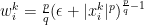
![\displaystyle 0 = \alpha \Big[\frac{p}{q} (\epsilon + |x_i|^q)^{\frac{p}{q}-1} q \textup{sgn}(x_i) |x_i|^{q-1}\Big]_i + A^*(Ax-b)](https://s0.wp.com/latex.php?latex=%5Cdisplaystyle+0+%3D+%5Calpha+%5CBig%5B%5Cfrac%7Bp%7D%7Bq%7D+%28%5Cepsilon+%2B+%7Cx_i%7C%5Eq%29%5E%7B%5Cfrac%7Bp%7D%7Bq%7D-1%7D+q+%5Ctextup%7Bsgn%7D%28x_i%29+%7Cx_i%7C%5E%7Bq-1%7D%5CBig%5D_i+%2B+A%5E%2A%28Ax-b%29+&bg=ffffff&fg=000000&s=0&c=20201002)
Note that the exponent 


![\displaystyle 0 = \alpha \Big[\frac{p}{q} (\epsilon + |x_i^k|^q)^{\frac{p}{q}-1} q \textup{sgn}(x_i) |x_i|^{q-1}\Big]_i + A^*(Ax-b)](https://s0.wp.com/latex.php?latex=%5Cdisplaystyle+0+%3D+%5Calpha+%5CBig%5B%5Cfrac%7Bp%7D%7Bq%7D+%28%5Cepsilon+%2B+%7Cx_i%5Ek%7C%5Eq%29%5E%7B%5Cfrac%7Bp%7D%7Bq%7D-1%7D+q+%5Ctextup%7Bsgn%7D%28x_i%29+%7Cx_i%7C%5E%7Bq-1%7D%5CBig%5D_i+%2B+A%5E%2A%28Ax-b%29+&bg=ffffff&fg=000000&s=0&c=20201002)
for 

Lai and Wang do this for 


Of course the question arises if there is a chance that the limit will be a global minimizer. Unfortunately this is not probable as a simple numerical experiment shows:
Example 2 We apply the iteration (5) to the one dimensional problem (3) in which we know the solution. We do this for many values of
, set
and chose
. This produced the following output (I plotted every fifth iteration):
Well, the iteration always chose the upper branch… In a second experiment I initialized with a smaller value, namely withfor all
That’s interesting: I ended at the upper branch for all values below the point where the lower branch (the one with the local maximum) crosses the initialization line. This seems to be true in general. Starting with
gave
Well, probably this is not too interesting: Starting “below the local maximum” will bring you to the local minimum which is lower and vice versa. Indeed Lai and Wang proved in their Theorem 2.5 that for a specific setting (small enough such that the method will pick the global minimizer. But wait—they do not say anything about initialization… What happens if we initialize with zero? I have to check…


By the way: A similar experiment as in this example with different values of
2. Iterative thresholding
Together with Kristian Bredies I developed another approach to these nasty non-convex minimization problems with 
Remark 1 When showing results for problems in separable Hilbert space I sometimes get the impression that others think this is somehow pointless since in the end one always works with
in practice. However, I think that working directly in a separable Hilbert space is preferable since then one can be sure that the results will not depend on the dimension
in any nasty way.
Basically our approach was, to use one of the most popular approaches to the 

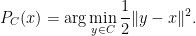
by the projected gradient method. That is: do a gradient step and use the projection 


Now note that the projection is characterized by
Now we replace the “convex constraint” 
Then, we just replace the minimization problem for the projection with
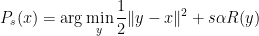
and iterate

The crucial thing is, that one needs global minimizers to obtain 

One easily proves that one gets descent of the objective functional:
Lemma 1 Let
with Lipschitz constant
and let
be weakly lower semicontinuous and coercive. Furthermore let
denote any solution of
Then for
it holds that


Proof: Start with the minimizing property

and conclude (by rearranging, expanding the norm-square, canceling terms and adding 

Finally, use Lipschitz-continuity of


This gives descent of the functional value as long as 
To make a long story short: For 


However, with considerably more effort one can show the following: For the iteration 

That’s not too bad yet. Currently Kristian and I, together with Stefan Reiterer, work to show that the whole sequence of iterates converges. Funny enough: This seems to be true for 
![{]0,1[}](https://s0.wp.com/latex.php?latex=%7B%5D0%2C1%5B%7D&bg=ffffff&fg=000000&s=0&c=20201002)

August 25, 2012 at 9:42 pm
[…] correctly, she also treated “iteratively reweighted least squares” as I described in my previous post. Unfortunately, she did not include the generalized forward-backward methods based on -functions […]